NoSQL
- Key-Value Stores
- Column-oriented Databases
- Document-oriented Databases
- Graph Databases
- Bibliography
Key-Value Stores
- Known databases: Riak, Redis, memcached, memcachedb, membase, Voldemort
- Not performant for complex queries and aggregate operations
Riak
- Riak is a distributed key-value database where values can be anything—from plain text, JSON, or XML to images or video clips—all accessible through a simple HTTP interface
- is a distributed, datareplicating, enhanced key-value store without a single point of failure
- Implementation of Amazon’s Dynamo
- Embraces web constructs of HTTP and REST from ground up
- supports advanced querying via mapreduce.
- Riak is a great choice for datacenters like Amazon that must serve many requests with low latency. If every millisecond spent waiting is a potential customer loss, Riak is hard to beat.
- Riak breaks up classes of keys into buckets to avoid key collisions.
- Riak stores everything as a binary-encoded value.
- Links are metadata that associate one key to other keys. Links are uni-directional. What makes Links special in Riak is link walking (and a more powerful variant, linked mapreduce queries)
- URL Pattern:
http://SERVER:PORT/riak/BUCKET/KEY.
Architecture
- Riak server architecture removes single points of failure (all nodes are peers) and allows you to grow or shrink the cluster at will. This is important when dealing with large-scale deployments, since it allows your database to remain available even if several nodes fail or are otherwise unresponsive.
- Riak takes advantage of this fact by allowing you to trade availability for consistency on a per-request basis.
- Riak Ring - Riak divides its server configuration into partitions denoted by a 160-bit number (that’s 2^160). The Riak team likes to represent this massive integer as a circle, which they call the ring. When a key is hashed to a partition, the ring helps direct which Riak servers store the value.
Clustering
- Riak allows us to control reads and writes into the cluster by altering three values:
Nis the number of nodes a write ultimately replicates to, in other words, the number of copies in the cluster.Wis the number of nodes that must be successfully written to before a successful response. IfWis less thanN, a write will be considered successful even while Riak is still copying the value in background.Ris the number of nodes required to read a value successfully. IfRis greater than the number of copies available, the request will fail. IfR=1, there is a potential chance to read stale values. IfR=N, then if any of thoseNnodes become unavailable, read requests would fail.
- Conflict Resolution
- Riak uses vector clocks. A vector clock is a token that distributed systems like Riak use to keep the order of conflicting key-value updates intact. Timestamps cannot be used since the clocks across servers may not be synchronized.
Downsides/Limitations/Trade-offs
- lacks robust support for ad hoc queries, and key-value stores, by design, have trouble linking values together (in other words, they have no foreign keys).
- If you require simple queryability, complex data structures, or a rigid schema or if you have no need to scale horizontally with your servers, Riak is probably not your best choice.
Redis
- Redis stands for Remote Dictionary Server
- provides for complex datatypes like sorted sets and hashes, as well as basic message patterns like publish-subscribe and blocking queues.
-
by caching writes in memory before committing to disk, Redis gains amazing performance in exchange for increased risk of data loss in the case of a hardware failure. good fit for caching noncritical data and for acting as a message broker.
- 3 Persistence modes
- in-memory - completely in-memory. data is lost when server crashes
- snapshot (default) - snapshots taken to files periodically
- Append Only File (AOF) - all data is written to file every few seconds
- Keys
- Redis keys can be a simple string or a complex string (e.g., persons:123:nyc)
- A key can be of max size 512 MB. Keep it simple and small for performance
- expiration time can be set on keys
- Key space and keys are like Databases and tables in RDBMS
Data Types
- Hash or Dictionaries
- Linked List
- Sets
- Max number of elements a set can hold is 2^32 -1 (around 4 billion)
- Sorted sets
- Each element is associated with a score. If 2 elements have same score, then they are sorted lexicographically in alphebetic order
- Useful to build applications like leaderboard
- Not as fast as sets since the scores are compared
- Add, remove and update of an item is
O(log N) - Internally sorted sets are implemented as 2 separate data structures
- A skip list with a hash table. A skip list is a data structure that allows fast search within an ordered sequence of elements.
- and a ziplist
- Bitmaps
- A Bitmap is not a real data type in Redis. Under the hood, a Bitmap is a String or a set of bit operations on a String.
- also known as bit arrays or bitsets.
- A Bitmap is a sequence of bits where each bit can store 0 or 1.
- Pro: are memory efficient, support fast data lookups, and can store up to 2^32 bits (more than 4 billion bits).
- Con: have to define the size of the bitmap upfront. e.g., if you are storing 5 million user ids, you have to define the bitmap of size 5m
- Con: not memory efficient, if only a fraction of those bits are actually being used
- HyperLogLogs
- A HyperLogLog is not actually a real data type in Redis. Conceptually, a HyperLogLog is an algorithm that uses randomization in order to provide a very good approximation of the number of unique elements that exist in a Set.
- It runs in
O(1)and uses a very small amount of memory—up to 12 kB of memory per key. - Redis provides specific commands to manipulate Strings in order to calculate the cardinality of a set using the HyperLogLog algorithm.
- The HyperLogLog algorithm is probabilistic, which means that it does not ensure 100 percent accuracy. The Redis implementation of the HyperLogLog has a standard error of 0.81 percent. In theory, there is no practical limit for the cardinality of the sets that can be counted.
- Commands for HyperLogLogs: PFADD, PFCOUNT, and PFMERGE. (PF stands for Philippe Flajolet, the author of the algorithm)
- Pro: Usually, to perform unique counting, you need an amount of memory proportional to the number of items in the set that you are counting. HyperLogLogs solve these kinds of problems with great performance, low computation cost, and a small amount of memory.
- Con: are not 100% accurate. Nonetheless, in some cases, 99.19 percent is good enough.
- Use cases where this can be useful
- Counting the number of unique users who visited a website
- Counting the number of distinct terms that were searched for on your website on a specific date or time
- Counting the number of distinct hashtags that were used by a user
- Counting the number of distinct words that appear in a book
Redis CLI
pingconfig- to view the configuration details fromredis.confset <key> <value>get <key>del <key>select <keyspace>- create or switch to a given key space (key space is a name space like db in rdbms)keys *- returns all keys in the current spaceflushdb- delete all keys in the key spaceexpire <key> <time_in_secs>- expires a key after given timettl <key>- shows the key’s time to live in secondspersist <key>- removes the timeout of a keysetex <key> <timeout> <value>- set value and timeout- Hash
hset <redis_key> <key> <value>- set a single key value in a redis keyhget <redis_key> <key> <value>- get a single key’s value from a redis keyhmset <redis_key> <key1> <value1> <key2> <value2>- set multiple key valueshmget<redis_key> <key1> <key2>- get multiple valueshgetall <redis_key>- returns all key values in this redis key
- Linked List
lpush <list_name> <value>- left push a value to listrpush <list_name> <value>- right push a value to listlrange <list_name> <from_index> <to_index>- returns all the elements in the list within the given rangelpop <list_name>- pop out the left most element from the listrpop <list_name>- pop out the right most element from the listllen <list_name>- length of the listltrim <list_name> <from_index> <to_index>- trims the elements off of the list that is within the range
- Set
sadd <set> <value>sunion <set1> <set2>- union of 2 setssinter <set1> <set2>- intersection of 2 setssdiff <set1> <set2>- difference of 2 setssismember <set> <value>- checks if the given value is a member of this setsmembers <set>- returns all the values/members from this setsrem <set> <value>- remove an element from the setscard <set>- cardinality of a set
- Sorted Set
zadd <set> <score> <value>- e.g.,zadd leaders 100 "Alice"zrange
Advanced Features
- Pub-Sub
- Redis support publish-subscribe pattern. Publishers send messages to channels, and subscribers receive these message if they are listening to a channel.
- Uses cases where Redis can be used as a pub-sub: News and weather dashboards, Chat apps, Push notifications such as travel alerts, Remote code execution similar to what the SaltStack tool supports.
- Transaction
- Redis supports atomic execution of a sequence of commands in a transaction.
MULTIstarts a transaction,EXECis commit,DISCARDis rollback
- Pipelines
- is a way to send multiple commands together to the Redis server without waiting for individual replies. The replies are read all at once by the client.
- commands are run sequentially in the server (the order is preserved), but they do not run as a transaction
- Pipelines can improve the network’s performance significantly.For instance, if the network link between a client and server has a round trip time of 100 ms, the maximum number of commands that can be sent per second is 10, no matter how many commands can be handled by the Redis server. Usually, a Redis server can handle hundreds of thousands of commands per second, and not using pipelines may be a waste of resources.When Redis is used without pipelines, each command needs to wait for a reply.
- Security
- Redis uses plain-text based passwords. Does not support ACLs.
- Redis is meant to run in a trusted network. To protect the servers running in a public cloud
- Use firewall rules to block access from unknown clients. Either setting
iptablesin linux directly or via Security Groups in AWS-like setting - Run Redis on the loopback interface (127.0.0.1), rather than a publicly accessible network interface. This applies only if the application server and the Redis server as running on the same machine.
- Run Redis in a virtual private cloud instead of the public Internet
- Encrypt client-to-server communication.
- Redis does not support encryption by default. A tool like
stunnelcan be used as an SSL encryption wrapper between a local client and a local or remote server. - There are 2 options for running Redis with stunnel:
- (1) Run stunnel on both the server and client machines, using the same private key:
- The stunnel in the server creates a tunnel to the redis-server
- The stunnel in the client creates a tunnel to the remote stunnel (on the server machine). The Redis client should connect to the local stunnel
- (2) Run stunnel on the server, and a Redis client that supports SSL must be used. This client will use the private key to encrypt the connection
- (1) Run stunnel on both the server and client machines, using the same private key:
- Redis does not support encryption by default. A tool like
- Use firewall rules to block access from unknown clients. Either setting
Scalability
Persistence
- 2 mechanisms of persistence: RDB (Redis Database) and Append-only File (AOF)
- RDB
SAVEcommand creates a LZF-compressed binary.rdbfile that has a point in time representing data.- great for backups and disaster recovery since it allows you to save a file every hour, day, week or month
- Redis uses copy-on-write mechanism to take backups
- When creating a snapshot, Redis main process executes a
fork()to create a child process which can make the Redis instance stop serving clients for milliseconds or seconds.
- AOF
- AOF is a human-readable append-only log file.
- AOF is an alternative to RDB snapshotting, but both can be used together. Redis will load RDB or AOF on startup if any of the files exists. If both files exist, the AOF takes precedence because of its durability guarantees.
- When AOF is enabled, every time Redis receives a command that changes the dataset, it will append that command to the AOF (Append-only File). With this being said, if you have AOF enabled and Redis is restarted, it will restore the data by executing all commands listed in AOF, preserving the order, and rebuild the state of the dataset.
- Restoring big dataset from an RDB is faster than AOF since RDB does not need to re-execute every change made
- Considerations when using persistence in Redis:
- If your application does not need persistence, disable RDB and AOF
- If your application has tolerance to data loss, use RDB
- If your application requires fully durable persistence, use both RDB and AOF
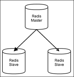
Replication
- a master can have multiple slaves and slaves can also accept connections from other slaves.
- Replicas are widely used for scalability purposes so that all read operations are handled by replicas and the master handles only write operations.
- Persistence can be moved to the replicas so that the master does not perform disk I/O operations. In this scenario, the master server needs to disable persistence, and it should not restart automatically for any reason; otherwise, it will restart with an empty dataset and replicate it to the replicas, making them delete all of their stored data.
- Data Consistency: It is possible to improve data consistency guarantees by requiring a minimum number of replicas connected to the master server. In this way, all write operations are only executed in the master Redis server if the minimum number of replicas are satisfied, along with their maximum replication lag (in seconds). However, this feature is still weak because it does not guarantee that all replicas have accepted the write operations; it only guarantees that there is a minimum number of replicas connected to the master.
- Replicas are very useful in a master failure scenario because they contain all of the most recent data and can be promoted to master. Unfortunately, when Redis is running in single-instance mode, there is no automatic failover to promote a slave to master. All replicas and clients connected to the old master need to be reconfigured with the new master.
Partitioning
- Redis does not natively support partitioning or clustering. It was designed to work well on a single server. Redis Cluster is designed to solve distributed problems in Redis.
- 2 types of partitioning: horizontal (sharding) and vertical partitioning
- Range partitioning
- e.g., user ids 1-1000 in one server, etc. Alphabet range where A-G in one instance, H-O in another, etc.
- Con: the distribution of data could be uneven
- Con: does not accommodate the change easily
- Hash partitioning
- Pro: data distribution is even
- Con: when new servers are added, data in other instances become invalidated.
- Con: adding or removing nodes from the list of servers may have a negative impact on key distribution and creation.
- Presharding
- One way of dealing with the problem of adding/replacing nodes over time with hash partitioning is to preshard the data. This means pre-partitioning the data to a high extent so that the host list size never changes. The idea is to create more Redis instances, reuse the existing servers, and launch more instances on different ports. This works well because Redis is single threaded and does not use all the resources available in the machine, so you can launch many Redis instances per server and still be fine.
- Then, with this new list of Redis instances, you would apply the same Hash algorithm that we presented before, but now with far more elements in the Redis client array.
- This method works because if you need to add more capacity to the cluster, you can replace some Redis instances with more powerful ones, and the client array size never changes.
- Consistent Hashing or Hash Ring
- If Redis is used as a cache system with hash partitioning, it becomes very hard to scale up because the size of the list of Redis servers cannot change (otherwise, a lot of cache misses will happen).
- Consistent hashing is a kind of
hashing that remaps only a small portion of the data to different servers when the list of Redis servers is changed (only
K/nkeys are remapped, whereKis the number of keys andnis the number of servers). - For example, in a cluster with 100 keys and four servers, adding a fifth node would remap only 25 keys on an average (100 divided by 4).
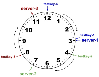
- The technique consists of creating multiple points in a circle for each Redis key and server. The appropriate server for a given key is the closest server to that key in the circle (clockwise); this circle is also referred to as “ring.” The points are created using a hash function, such as MD5.
- More on consistent hashing: link 1
- Tagging
- is a technique of ensuring that keys are stored on the same server. Commands such as
SDIFF,SINTER, andSUNIONrequire that all keys are stored in the same Redis instance in order to work. - One way of guaranteeing that the keys will be stored in the same Redis instance is by using tagging.
- Choose a convention for your key names and add a prefix or suffix. Then decide how to route that key based on the added prefix or suffix. The convention in the Redis community is to add a tag to a key name with the tag name inside curly braces (that is,
key_name:{tag}). * When Redis is used as a data store, the keys must always map to the same Redis instances and tagging should be used. Unfortunately, this means that the list of Redis servers cannot change; otherwise, a key could have been able to map to a different Redis instance. One way of solving this is to create copies of the data across Redis instances so that every key is replicated to a number of instances, and the system knows how to route queries (this is similar to how Riak stores data).
- is a technique of ensuring that keys are stored on the same server. Commands such as
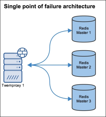
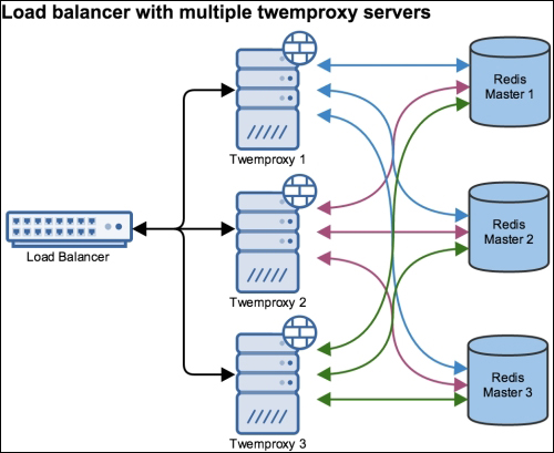
Automatic Sharding with twemproxy
- also known as nutcracker
- twemproxy is a fast and lightweight proxy developed by Twitter for Redis and memcached protocols that implements sharding with support for multiple hashing modes, including consistent hashing.
- It also enables pipelining of requests and responses, and maintains persistent server connections to shard your data automatically across multiple servers.
- it will help us easily scale Redis horizontally.
- It has been used in production by companies such as Pinterest, Tumblr, Twitter, Vine, Wikimedia, Digg, and Snapchat.
Architecture styles using twemproxy
| Single point of failure architecture | Load balance with multiple twemproxy servers |
|---|---|
 |
 |
Redis Sentinel
- Redis Sentinel is a distributed system designed to automatically promote a Redis slave to master if the existing master fails.
- Sentinel does not distribute data across nodes since the master node has all of the data and the slaves have a copy of the data
- Sentinel is not a distributed data store.
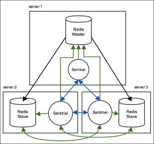
- The most common architecture contains an installation of one Sentinel for each Redis server.
- Sentinel is a separate process from the Redis server, and it listens on its own port.
- A client always connects to a Redis instance, but it needs to query a Sentinel to find out what Redis instance it is going to connect to.
- Client tries to connect to one of the sentinels in the configuration. If the first sentinel is down, it moves on to the next until it can find a sentinel which tells who is the current master.
- When you download Redis, it comes with a configuration file for Sentinel, called
sentinel.conf. In the initial configuration, only the master nodes need to be listed. All slaves are found when Sentinel starts and asks the masters where their slaves are. - The Sentinel configuration will be rewritten as soon as the Sentinel finds all the available slaves, or when a failover occurs.
- Communication between all Sentinels takes place through a Pub/Sub channel called
__sentinel__:helloin the Redis master.
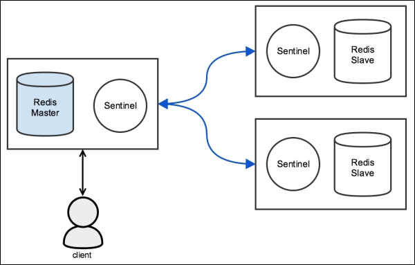
| Redis without Sentinel | Redis with Sentinel |
|---|---|
 |
 |
Configuration
1 2 3 4 | |
- The preceding configuration monitors a Redis master with the name mymaster, IP address 127.0.0.1, port 6379, and quorum 2.
- The quorum represents the fewest number of sentinels that need to agree that the current master is down before starting a new master election.
- A Sentinel will only notify other Sentinels that its master is down after the master is unreachable (unable to reply a PING) for a given number of milliseconds, specified in the directive
down-after-milliseconds. - The sentinel configuration is rewritten every time a new master is elected or a new sentinel or slave joins the group of instances.
- Directive failover-timeout is to avoid a failover to a master that has experienced issues in a short period of time (which is specified via the failover-timeout directive). For example, assume that there is a master, R1, with three slaves, R2, R3, and R4. If the master experiences issues, the slaves need to elect a new master. Assume that R2 becomes the new master and R1 returns to the group as a slave. If R2 has issues and another new election must take place before failover-timeout is exceeded, R1 will not be part of the possible nodes to be elected as the master.
- parallel-syncs specifies the number of slaves that can be reconfigured simultaneously to point to a new master. During this process the slaves will be unavailable to clients. Use a low parallel-syncs number to minimize the number of simultaneously unavailable slaves.
Network Partition (split-brain)
| Redis without Sentinel | Redis with Sentinel |
|---|---|
 |
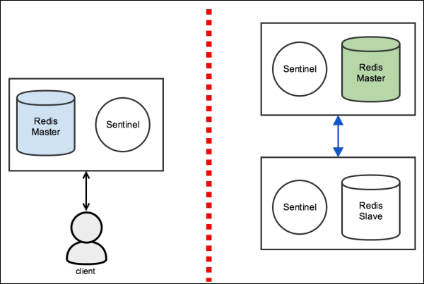 |
- Redis Sentinel is not strongly consistent in a network partition scenario. Data may be lost when a split-brain occurs.
- Kyle Kingsbury (also known as Aphyr on the Internet) wrote some very detailed blog posts on Redis Sentinel and its lack of consistency. The last post can be found at https://aphyr.com/posts/287-asynchronous-replication-with-failover.
- Salvatore Sanfilippo (also known as Antirez) wrote a reply to that blog post, which can be found at http://antirez.com/news/56.
To demonstrate how Redis Sentinel will lose data when a split-brain occurs, assume the following:
There are three Redis instances: one master and two replicas. For each Redis instance, there is a Redis Sentinel There is a client connected to the current master and writing to it If a network partition occurs and separates the current master from all of its slaves, and the slaves can still talk to each other, one of the slaves will be promoted to master.
Meanwhile, the client will continue to write to the isolated master.
If the network heals and all the servers are able to communicate to each other again, the majority of sentinels will agree that the old master (the one that was isolated) should become a slave of the new master (the slave that was promoted to master). When this happens, all writes sent by the client are lost, because there is no data synchronization in this process.
Redis Cluster
- Redis Cluster was designed to automatically shard data across different Redis instances, providing some degree of availability during network partitions. It is not strongly consistent under chaotic scenarios.
- Unlike Sentinel, Redis Cluster only requires a single process to run but requires two ports:
- The first is used to serve clients (low port), and
- the second serves as a bus for node-to-node communication (high port). The high port is used to exchange messages such as failure detection, failover, resharding, and so on.
The Redis Cluster bus uses a binary protocol to exchange messages between nodes. The low port is specified in the configuration, and Redis assigns the high port by adding 10,000 to the low port. For example, if a Redis server starts listening to port 6379 (low port) in cluster mode, it will internally assign port 16379 (high port) for node-to-node communication. The Redis Cluster topology is a full mesh network. All nodes are interconnected through Transmission Control Protocol (TCP) connections.
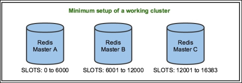
- Redis Cluster requires at least three masters, as shown in the following figure, to be considered healthy. All data is sharded across the masters and replicated to the slaves
- It is recommended that you have at least one replica per master. Otherwise, if any master node without at least one replica fails, the data will be lost
- Unlike Redis Sentinel, when a failover is happening in Redis Cluster, only the keys in the slots assigned to the failed master are unavailable until a replica is promoted. The data may be unavailable during a failover, because slave promotion is not instantaneous.
When Redis is in cluster mode, its interface is slightly changed. This requires a smarter client. When connecting to Redis through redis-cli, the -c parameter is required to enable cluster mode. Otherwise, Redis will work in single-instance mode:
$ redis-cli -c -h localhost -p 6379
- To try out: Redis Labs or try.redis
Column-oriented Databases
Overview
- Known databases: HBase, Cassandra, Hypertable
- Large data stored across machines, less data relationships
- adding columns is quite inexpensive
- Each row can have a different set of columns, or none at all, allowing tables to remain sparse without incurring a storage cost for null values.
HBase
- Using Google’s BigTable paper as a blueprint, HBase is built on Hadoop (a mapreduce engine) and designed for scaling horizontally on clusters of commodity hardware.
- supports versioning and compression.
- HBase is a column-oriented database that prides itself on consistency and scaling out.
- A table in HBase is basically a big map. Well, more accurately, it’s a map of maps.
- Unlike a relational database, in HBase a column is specific to the row that contains it. When we start adding rows, we’ll add columns to store data at the same time.
- HBase stores an integer timestamp for all data values, representing time in milliseconds since the epoch (00:00:00 UTC on January 1, 1970). When a new value is written to the same cell, the old value hangs around, indexed by its timestamp. This is a pretty awesome feature. Most databases require you to specifically handle historical data yourself, but in HBase, versioning is baked right in!
- A Bloom filter is a really cool data structure that efficiently answers the question, “Have I ever seen this thing before?”. HBase supports using Bloom filters to determine whether a particular column exists for a given row key (BLOOMFILTER=>’ROWCOL’) or just whether a given row key exists at all (BLOOMFILTER=>’ROW’). The number of columns within a column family and the number of rows are both potentially unbounded. Bloom filters offer a fast way of determining whether data exists before incurring an expensive disk read.
- In HBase, rows are kept in order, sorted by the row key. A region is a chunk of rows, identified by the starting key (inclusive) and ending key (exclusive). Regions never overlap, and each is assigned to a specific region server in the cluster.
Why use HBase?
Scalability, built-in features like versioning, compression, garbage collection of expired data, in-memory tables. Strong consistency guarantees makes it easier to transition from relational world.
Where to use?
- Best used for online analytical processing systems - though individual queries are slower compared to other dbs, it works really well with enormous datasets. Big companies use this to back logging and search systems. Used by Facebook a principal component of its new messaging infrastructure. Twitter uses HBase extensively, ranging from data generation (for applications such as people search) to storing monitoring/performance data
Architecture
- HBase is designed to be fault tolerant. Hardware failures may be uncommon for individual machines, but in a large cluster, node failure is the norm. By using write-ahead logging and distributed configuration, HBase can quickly recover from individual server failures.
- HBase supports three running modes:
- Stand-alone mode is a single machine acting alone.
- Pseudodistributed mode is a single node pretending to be a cluster.
- Fully distributed mode is a cluster of nodes working together.
Downsides
- Although HBase is designed to scale out, it doesn’t scale down.
- Solving small problems isn’t what HBase is about, and nonexpert documentation is tough to come by, which steepens the learning curve.
- HBase is almost never deployed alone. Rather, it’s part of an ecosystem of scale-ready pieces. These include Hadoop (an implementation of Google’s MapReduce), the Hadoop distributed file system (HDFS), and Zookeeper (a headless service that aids internode coordination). This ecosystem is both a strength and a weakness; it simultaneously affords a great deal of architectural sturdiness but also encumbers the administrator with the burden of maintaining it.
- One noteworthy characteristic of HBase is that it doesn’t offer any sorting or indexing capabilities aside from the row keys. Rows are kept in sorted order by their row keys, but no such sorting is done on any other field, such as column names and values. So, if you want to find rows by something other than their key, you need to scan the table or maintain your own index.
- There is no concept of data types. Everything is an uninterrupted array of bytes
Document-oriented Databases
MongoDB
- supports consistency. Supports ACID properties at single-document level only.
- offers atomic read-write operations such as incrementing a value and deep querying of nested document structures.
- Using JavaScript for its query language, MongoDB supports both simple queries and complex mapreduce jobs.
- It is a document database, which allows data to persist in a nested state, and importantly, it can query that nested data in an ad hoc fashion. It enforces no schema.
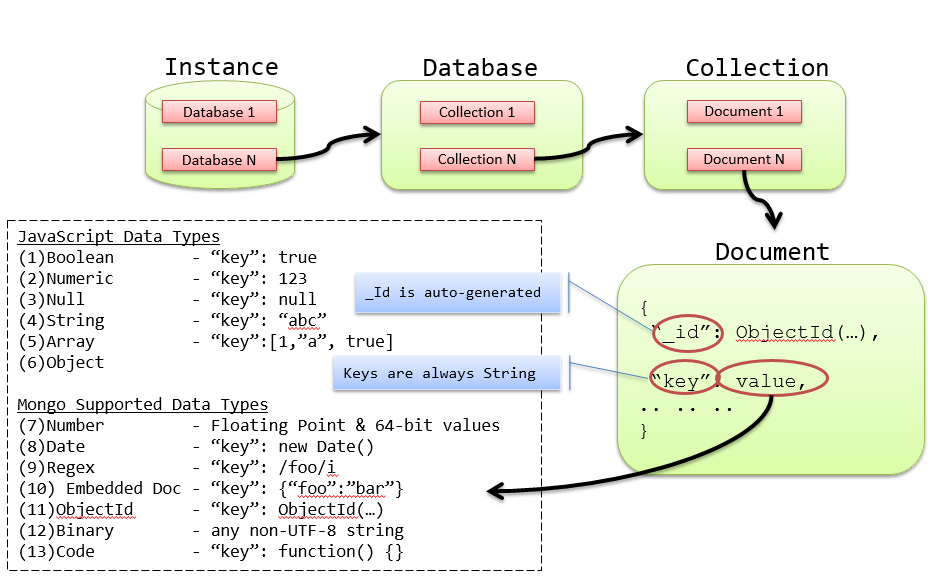
- Mongo is a JSON document database (though technically data is stored in a binary form of JSON known as BSON).
- Every object/document has a unique incrementing numeric primary key called ObjectId. The ObjectId is always 12 bytes, composed of a timestamp, client machine ID, client process ID, and a 3-byte incremented counter.
- In Mongo you can construct ad hoc queries by field values, ranges, or a combination of criteria.
- MongoDB provides several of the best data structures for indexing, such as the classic B-tree, and other additions such as two-dimensional and spherical GeoSpatial indexes.
- What makes Mongo special in the realm of document stores is its ability to scale across several servers, by replicating (copying data to other servers) or sharding collections (splitting a collection into pieces) and performing queries in parallel. Both promote availability.
- A Namespace in Mongo is a combination of database name and collection name. e.g.,
db.plans - GridFS
Index
- By default, MongoDB creates an index on the document’s _id primary key field.
- All user-defined indexes are secondary indexes. Any field can be used for a secondary index, including fields within arrays
- Order of columns on the compound index matters
- Use
explain()to analyze the performance of a query.db.plans.find({"clientId" : "014222"}).explain() - Use the
hint()method to tell Mongo which index to use.
Index Types
- Unique indexes
- Array indexes - For fields that contain an array, each array value is stored as a separate index entry. There is no special syntax for array indexes though.
- Sparse Indexes - Sparse indexes only contain entries for documents that contain the specified field. Because MongoDB’s allows the data model to vary from one document to another, it is common for some fields to be present only in a subset of all documents. Sparse indexes allow for smaller, more efficient indexes when fields are not present in all documents.
- Hash Indexes - Hash indexes compute a hash of the value of a field and index the hashed value. The primary use of this index is to enable hash-based sharding, a simple and uniform distribution of documents across shards
- Capped collection - max size of the collection is defined at the time of creation and cannot be altered; an existing regular collection can be converted to capped collection, but not vice versa. It behaves like a circular queue and maintains the insertion order; cannot be sharded.
- Tailable cursors - like
tail -fcommand, tailable cursors can be defined on capped collections. - TTL indexes - Time-to-Live indexes are customizable capped collections where time-out for each document is defined by the user. A common use is in applications that maintain a rolling window of history (e.g., most recent 100 days) for user actions such as clickstreams.
- Full-text indexes - give you the ability to search text quickly, as well as provide built-in support for multi-language stemming and stop words; only index string data; allows searching multiple fields with custom weightage specified (from default 1 to 1 billion); You can create a full-text index on all string fields in a document by creating an index on
$** - Geo-spatial indexes
- Types of Geospatial queries : intersection, within, and nearness; Geospatial queries using intersection and within functions do not require an index, whereas near function does.
- 2dsphere index - for surface-of-the-earth-type maps; allows you to specify points, lines, and polygons in GeoJSON format. A point is given by a two-element array, representing [longitude, latitude]; A line by an array of Points; A polygon in the same way as lines but with different ‘type’; Sample queries: restaurants in given coordinates, restaurants near given coordinates.
- 2d index - for flat maps, video game maps and time series data; “2d” indexes assume a perfectly flat surface, instead of a sphere; can only store points;
Rules of Index Design
- Any fields that will be queried by equality should occur first in the index definition.
- Fields used to sort should occur next in the index definition. If multiple fields are being sorted (such as (last_name, first_name), then they should occur in the same order in the index definition.
- Fields that are queried by range should occur last in the index definition.
Profiling
- MongoDB provides a range of logging and monitoring tools to ensure collections are appropriately indexed and queries are tuned.
- The MongoDB Database Profiler is most commonly used during load testing and debugging, logging all database operations or only those events whose duration exceeds a configurable threshold (the default is 100ms).
- Profiling data is stored in a capped collection
Data modelling
Tips
- Embed for speed, reference for integrity
- Embed “point-in-time” data. E.g., the address fields in an order document. You don’t want a user’s past orders to change if he updates his profile.
- Do not embed fields that have unbound growth. e.g, comments on a blog article.
- Store embedded information in arrays for anonymous access. Subdocument should be used only when you know and will always know the name of the field that you are accessing.
Embedded document model
- Pros
- Locality. Less disk seeks and hence faster.
- Atomicity & Isolation during mutant operations.
- Cons
- Querying for all sub-documents with a matching condition would return the sub-document along with parent as well. Major drawback of this approach is that we get back much more data than we actually need.
- For example, in a document like below, querying for all the comments by John would return all the books where John has commented, not just the comments. Also it is not possible to sort or limit the comments returned.
1 2 3 4 5 6 7 8 9 | |
- Embedding carries significant penalties with it:
- The larger a document is, the more RAM it uses.
- Growing documents must eventually be copied to larger spaces. As you append to the large document, eventually MongoDB is going to need to move the document to an area with more space available. This movement, when it happens, significantly slows update performance
- MongoDB documents have a hard size limit of 16 MB.
- When to use
- If your application’s query pattern is well-known and data tends to be accessed in only one way, an embedded approach works well.
Referenced document model
- Pros
- Flexibility
- Best fit for many-to-many relationships.
- Cons
- No joins hence needs multiple network calls to retrieve complete data.
- There is no multi-document transaction in Mongodb. In other words, unlike SQL you cannot edit/delete multiple documents in a single transaction. If a business entity spans across multiple collections, you cannot alter that entity from different collections atomically.
- When to use
- If your application may query data in many different ways, or you are not able to anticipate the patterns in which data may be queried, a more “normalized” approach may be better.
- Another factor that may weigh in favor of a more normalized model using document references is when you have one-to-many relationships with very high or unpredictable arity.
Transaction Management
- MongoDB write operations are atomic at the document level – including the ability to update embedded arrays and sub-documents atomically
- Document-level atomicity in MongoDB ensures complete isolation as a document is updated
- Multi-document transaction
findAndModify()command that allows a document to be updated atomically and returned in the same round trip. Will this work for multiple documents?- For situations that require multi-document transactions, you can implement two-phase commit in your application to provide support for these kinds of multi-document updates. Using 2 Phase Commit ensures that data is consistent and, in case of an error, the state that preceded the transaction is recoverable. During the procedure, however, documents can represent pending data and states.
- Maintaining Strong Consistency - By default, MongoDB directs all read operations to primary servers, ensuring strong consistency. Also, by default any reads from secondary servers within a MongoDB replica set will be eventually consistent – much like master / slave replication in relational databases.
- Write concerns - The write concern is configured in the driver and is highly granular – it can be set per-operation, per-collection or for the entire database.
- Journals
- Before applying a change to the database – whether it is a write operation or an index modification – MongoDB writes the change operation to the journal. If a server failure occurs or MongoDB encounters an error before it can write the changes from the journal to the database, the journaled operation can be reapplied, thereby maintaining a consistent state when the server is recovered.
Why no transactions?
- MongoDB was designed from the ground up to be easy to scale to multiple distributed servers. Two of the biggest problems in distributed database design are distributed join operations and distributed transactions.
- Both of these operations are complex to implement, and can yield poor performance or even downtime in the event that a server becomes unreachable. By “punting” on these problems and not supporting
Write concern
- MongoDB has a configurable write concern. This capability allows you to balance the importance of guaranteeing that all writes are fully recorded in the database with the speed of the insert.
- For example, if you issue writes to MongoDB and do not require that the database issue any response, the write operations will return very fast (since the application needs to wait for a response from the database) but you cannot be certain that all writes succeeded. Conversely, if you require that MongoDB acknowledge every write operation, the database will not return as quickly but you can be certain that every item will be present in the database.
- The proper write concern is often an application-specific decision, and depends on the reporting requirements and uses of your analytics application.
Insert acknowledgement
By setting w=0, you do not require that MongoDB acknowledge receipt of the insert. db.events.insert(event, w=0)
Journal write acknowledgement
If you want to ensure that MongoDB not only acknowledges receipt of a write operation but also commits the write operation to the on-disk journal before returning successfully to the application, you can use the j=True option: db.events.insert(event, j=True).
MongoDB uses an on-disk journal file to persist data before writing the updates back to the “regular” data files. Since journal writes are significantly slower than in-memory updates (which are, in turn, much slower than “regular” data file updates), MongoDB batches up journal writes into “group commits” that occur every 100 ms unless overridden in your server settings. What this means for the application developer is that, on average, any individual writes with j=True will take around 50 ms to complete, which is generally even more time than it would take to replicate the data to another server.
Replication acknowledgement
To acknowledge that the data has replicated to two members of the replica set before returning: db.events.insert(event, w=2).
Aggregation Framework
- a pipeline that processes a stream of documents through several building blocks: filtering, projecting, grouping, sorting, limiting, and skipping.
aggregate()function returns an array of result documents; cannot write to a collection;- Pipeline Operations - Each operator receives a stream of documents, does some type of transformation on these documents, and then passes on the results of the transformation. If it is the last pipeline operator, these results are returned to the client. Otherwise, the results are streamed to the next operator as input.
Sharding
- One of the central reasons for Mongo to exist is to safely and quickly handle very large datasets. The clearest method of achieving this is through horizontal sharding by value ranges—or just sharding for brevity. Rather than a single server hosting all values in a collection, some range of values are split (or in other words, sharded) onto other servers. For example, in our phone numbers collection, we may put all phone numbers less than 1-500-000-0000 onto Mongo server A and put numbers greater than or equal to 1-500-000-0001 onto a server B. Mongo makes this easier by autosharding, managing this division for you.
- Diff b/w sharding and replication? Replication copies the exact copy of a data in multiple servers. Sharding stores different subset of data across multiple servers.
- Shard - server participating in a sharded cluster.
- mongos - routing process which sits in front of all the shards. Apps connect to this process.
- Sharding is enabled at database level.
-
Shard key - when you enable sharding you choose a field or two that MongoDb uses to break up data. To even create a shard key, the field(s) must be indexed. Before sharding, the collection is essentially a single chunk. Sharding splits this into smaller chunks based on the shard key
- Shard
- A shard is one or more servers in a cluster that are responsible for some subset of the data. For instance, if we had a cluster that contained 1,000,000 documents representing a website’s users, one shard might contain information about 200,000 of the users.
- A shard can consist of many servers. If there is more than one server in a shard, each server has an identical copy of the subset of data (Figure 2-1). In production, a shard will usually be a replica set.
- Single range shards will lead to cascade effect and lot of data movement when rebalancing is required. Mongo uses multi-range shards to avoid this.
- Chunk
- A range of data is called a chunk. When we split a chunk’s range into two ranges, it becomes two chunks.
- 200MB is the max size of a chunk by default. This is because moving data is expensive: it takes a lot of time, uses system resources, and can add a significant amount of network traffic.
- Shard Key
- You also cannot change the value of a shard key (with, for example, a $set). The only way to give a document a new shard key is to remove the document, change the shard key’s value on the client side, and reinsert it.
- A document belongs in a chunk if and only if its shard key value is in that chunk’s range.
- mongos
mongosis a special routing process that sits in front of your cluster and looks like an ordinarymongodserver to anything that connects to it. It forwards requests to the correct server or servers in the cluster, then assembles their responses and sends them back to the client. This makes it so that, in general, a client does not need to know that they’re talking to a cluster rather than a single server.- Targeted Query - While querying, if the query has the shard key, mongos determines which shard/shards contains the data and hits those directly. This is called a targeted query.
- Spewed Query - If the shard key is absent in the query, mongos must send the query to all of the shards. This can be less efficient than targeted queries, but not necessarily. A “spewed” query that accesses a few indexed documents in RAM will perform much better than a targeted query that has to access data from disk across many shards (a targeted query could hit every shard, too)
- Anatomy of a cluster
- A MongoDB cluster basically consists of three types of processes:
- the shards for actually storing data,
- the mongos processes for routing requests to the correct data, and
- the config servers, for keeping track of the cluster’s state
- A MongoDB cluster basically consists of three types of processes:
- Replica Sets
- Mongo was built to scale out, not to run stand-alone. It was built for data consistency and partition tolerance, but sharding data has a cost: if one part of a collection is lost, the whole thing is compromised. What good is querying against a collection of countries that contains only the western hemisphere? Mongo deals with this implicit sharding weakness in a simple manner: duplication. You should rarely run a single Mongo instance in production but rather replicate the stored data across multiple services.
- Partition
- Cluster has 1 or more shards
- Shard has 1 or more servers
- Shard has 1 or more chunks
- Chunk has 1 range
- Replica set
Setup
- To add configuration servers to router -
$mongos --configdb cfg-server1,cfg-server2,cfg-server3- All administration on a cluster is done through mongos
- Configuration servers can be 1, 2 or 3 max. They only have configuration information and no data.
- To add a shard -
db.runCommand({"addShard" : "server:port", "name": "shardName"})- Run this from the admin db
- To enable sharding at database level -
db.adminCommand({"enableSharding" : "dbname"}) - To enable sharding at collection level -
db.adminCommand({"shardCollection" : "dbname.collectionName", key : {"field1" : 1, "field2" : 1}}- If we are sharding a collection with data in it, the data must have an index on the shard key.
- All documents must have a value for the shard key, too (and the value cannot be null). After you’ve sharded the collection, you can insert documents with a null shard key value.
- To remove a shard out of the cluster -
db.runCommand({removeShard : "shardName"})- Moves all of the information that was on this shard to other shards before it can remove this shard.
- Moving data from shard to shard is pretty slow.
Shard Keys
- Bad shard keys
- Low cardinality keys
- e.g., by continent names, by country names, etc.
- When the volume increases in one of these shards, there is no way to horizontally scale because there are only limited number of key values.
- If you are tempted to use low-cardinality shard key because you query on that field a lot, use a compound shard key (a shard key with two fields) and make sure that the second field has lots of different values MongoDB can use for splitting.
- If a key has N values in a collection, you can only have N chunks and, therefore, N shards.
- Ascending Shard key
- e.g., timestamps, ObjectIds, auto-incrementing primary keys
- Everything will always be added to the “last” chunk, meaning everything will be added to one shard. This shard key gives you a single, undistributable hot spot.
- If the key’s values trend towards infinity, you will have this problem.
- Random Shard Key
- Low cardinality keys
- Good shard keys - Ideally, your shard key should have two characteristics:
- Insertions are balanced between shards
- Most queries can be routed to a subset of the shards to be satisfied
Sharding concerns
In a sharded environment, the limitations on the maximum insertion rate are:
- The number of shards in the cluster
-
The shard key you choose
- Limitations
- Cannot guarantee uniqueness on any key other than the shard key
- count of collection may return incorrect numbers
CouchDb
- Written in Erlang
- With nearly incorruptible data files, CouchDB remains highly available even in the face of intermittent connectivity loss or hardware failure.
- Like Mongo, CouchDB’s native query language is JavaScript.
- Storage data format: JSON
Admin UI
- Futon is a web-based interface to work with CouchDB and it provides support for editing the configuration information, creating databases, documents, design documents, etc.
- URI: http://localhost:5984/_utils/index.html
- How to create our first database? * Futon -> Overview -> Create database* . Multiple such databases can be created in this single instance of CouchDb.
How to access CouchDB programmatically?
via HTTP REST Interface
Note: If the db is password protected, send requests with credentials as follows: http://username:pass@remotehost:5984/dbname
- To check if the CouchDb is up and running:
curl http://localhost:5984 - To create a db:
- Request:
curl -X PUT http://localhost:5984/dbname - Response:
{"ok":true}
- Request:
- To delete a db:
- Request:
curl -X DELETE http://localhost:5984/dbname - Response:
{"ok":true}
- Request:
- To retrieve db information:
- Request:
curl -X GET http://localhost:5984/dbname - Response:
{"db_name":"dbname","doc_count":0,"doc_del_count":0,"update_seq":0,"purge_seq":0,"compact_running":false,"disk_size":79,"data_size":0,"instance_start_time":"1386975670043000","disk_format_version":6,"committed_update_seq":0}
- Request:
- To create a new document:
- Request:
curl -H "Content-type: application/json" -X POST http://localhost:5984/dbname -d "{\"title\": \"Lasagne\"}" - Response:
{"ok":true,"id":"d02bdee238b26628d1ce28f1c80313bb","rev":"1-f07d272c69ca1ba91b94544ec8eda1b6"} - Comments: ‘id’ is a unique document identifier and “rev” is the revision id of the document automatically generated.
- Request:
- To create a document with custom document id:
- Request:
curl -H "Content-type: application/json" -X PUT http://localhost:5984/dbname/pasat -d "{\"title\": \"Pasat\"}" - Response:
{"ok":true,"id":"pasat","rev":"1-91b034b589017f930d12f7fec23be727"} - Comments: PUT method is used instead of POST. Custom document id is passed in the url.
- Request:
- To retrieve a document:
- Request:
curl -X GET http://localhost:5984/dbname/d02bdee238b26628d1ce28f1c80313bb - Response:
{"_id":"d02bdee238b26628d1ce28f1c80313bb","_rev":"1-f07d272c69ca1ba91b94544ec8eda1b6","title":"Lasagne"} - Comments: Document ID is passed in the request.
- Request:
- To update a document:
- Request:
curl -H "Content-type: application/json" -X PUT http://localhost:5984/dbname/pasat -d "{\"title\": \"Fizal\", \"dob\": \"01/01/1980\", \"_rev\": \"1-91b034b589017f930d12f7fec23be727\"}" - Response:
{"ok":true,"id":"pasat","rev":"2-a294dbbe4a308e8586be9acdc527e6dc"} - Comments: Both doc id and rev id is needed to update a document. Updating the document means updating the entire document. You cannot add a field to an existing document. You can only write an entirely new version of the document into the database with the same document ID.
- Request:
- To delete a document:
- Request:
curl -H "Content-type: application/json" -X DELETE http://localhost:5984/dbname/pasat?rev=2-a294dbbe4a308e8586be9acdc527e6dc - Response:
{"ok":true,"id":"pasat","rev":"3-fc5a45ddd7178ee92532095c38d66489"} - Comments: Both doc id and rev id is needed to delete a document. Note that a new revision is created after deleting the document for replication purposes.
- Request:
- To upload attachments to a document:
- Request:
- To make a copy of a document:
- Request:
curl -X COPY ...
- Request:
- To request a UUID:
- Request:
curl -X GET http://localhost:5984/_uuids - Response:
{"uuids":["d02bdee238b26628d1ce28f1c803304f"]}
- Request:
- To compact a database:
Other Administration Tasks
- UI Set up
- To make Futon accessible outside of the localhost: Futon -> configurations -> Bind_Address - change the value to 0.0.0.0
- User Set up
- After set up, CouchDb runs in ‘Admin Party Mode’ (anyone accessing has full admin rights). To create an admin user and password, click on ‘Fix me’ link at the bottom right corner in Futon. The new admin user id should be visible under http://localhost:5984/_utils/database.html?_users.
- About Authentication: Couch has a pluggable authentication mechanism. Futon exposes a user friendly cookie-auth which handles login and logout.
- Database Set up
- How to create our first database? Futon -> Overview -> Create database
- Replication Set up
- How to replicate contents from DbX to DbY? Futon -> Tools -> Replicator -> Select from and to databases, and check the ‘Continuous’ checkbox. If the target db requires authentication, specify the url as http://username:pass@remotehost:5984/DbY.
Graph Databases
Concepts
Types of technologies in Graph space
- Graph Databases - Technologies used primarily for transactional online graph persistence, typically accessed directly in real time from an application. They are the equivalent of “normal” OLTP databases in the relational world. * Available Graph Dbs: Dex, FlockDB (Twitter), HyperGraphDb, InfiniteGraph, Neo4j, OrientDB, Titan, Microsoft Trinity.
- Graph Compute Engines - Technologies used primarily for offline graph analytics, typically performed as a series of batch steps. They are lik eother technologies for analysis of data in bulk, such as data mining and OLAP.
* Available Graph Compute Engines:
- In-memory/Single machine: Cassovary
- Distributed: Pegasus, Giraph
Graph databases either use a native graph storage or a non-native storage back-end (say a relational db). The benefit of a native graph storage is that its purpose-built stack is engineered for performance and scalability. The benefit of a non-native graph storage is the ease of use in production by the operation teams.
Advantages of Graph Databases
- Performance - In relation dbs, join across multiple tables is complex and tend to slow down with higher volume. In graph db, it is pretty much remains constant.
- Flexible data model: Adding new nodes, subgraphs and relations is lot easier and less intrusive than in relational model. No need to change the schema or the existing queries.
- Schemas are both rigid and brittle. Modifying schema often for business requirements is not an easy change. Creating a generic schema would end up with sparsely populated tables with many nullable columns. Vertical schemas add computational complexity in querying.
- Recursive questions such as “which customers bought this product who also bought that product?” is easy to write in graph model compared to relational.
- Pattern matching queries - e.g.?
- Geospatial queries - e.g.,?
Graph Data Models
- (1) Property graph model
- A property graph has the following characteristics:
- It contains nodes and relationships
- Nodes contain properties (key-value pairs)
- Relationships are named and directed, and always have a start and end node
- Relationships can also contain properties
- (2) RDF Triples - http://en.wikipedia.org/wiki/Resource_Description_Framework
- (3) Hypergraphs
- Graph Query Languages: Cypher (Neo4j), SPARQL (RDF query language), Gremlin (Imperative, path-based language)
- Graph Db Applications
- Recommendation Engines - e.g.,?
- Geospatial apps - e.g.,? Datastructure behind geospatial processing is R-tree. http://en.wikipedia.org/wiki/R-tree
Neo4j
http://nosql.mypopescu.com/tagged/neo4j
RDBMS is optimized for aggregated data. Neo4j is optimized for highly connected data.
- Cypher
- Get all node names –>
START n=node(*) RETURN n; - Get all nodes with rels –>
START n=node(*) MATCH n-[r?]-() RETURN n, r; - Delete all nodes –>
START n=node(*) MATCH n-[r?]-() DELETE n, r; - Query index –>
START n=node:TASK_NAME('TASK_NAME:("Task1", "Task2", "Task3")') RETURN n;
- Get all node names –>
Bibliography
- Seven Databases in Seven Weeks
- Graph Databases - O’Reilly
- http://nosql.findthebest.com/
- http://www.slideshare.net/samof76/distributed-keyvalue-stores-featuring-riak
- MongoDb
- MongoDb - The Definitive Guide
- MongoDB Applied Design Patterns
- Scaling Mondodb
- 50 Tips & Tricks for MongoDb Developers
- CouchDb
- Redis
- Redis Essentials
- Mastering Redis