RDBMS Concepts
- Keys
- Integrity
- Table Types
- Views
- Cursors
- Triggers
- Joins
- Administration Concepts
- Operational Commands
- Bibliography
Keys
Refer to SQL Tips and Techniques-2002
- Primary Key
- PK is an attribute or a set of attributes that uniquely identify a specific instance of an entity.
- PKs enforce entity integrity by uniquely identifying entity instances.
- Candidate Key - an entity can have more than one attribute that can serve as a primary key. Any key or minimum set of keys that could be a primary key is called a candidate key. (Eg. EmpId, SSN, Name of an Employee entity)
- Alternate Key - Rest of the non-primary keys are called alternate keys
- Composite Key - A primary key made up of more than one attribute is known as a composite key
- Foreign Key
- is an attribute that completes a relationship by identifying the parent entity.
- Foreign keys provide a method for maintaining integrity in the data (called referential integrity) and for navigating between different instances of an entity.
- Surrogate Key - system generated unique identifier. Not derived from application data.
- UUID or GUID or Object Id (as in Mongo)
- Sybase identity column
IDENTITY - Oracle
SEQUENCEorGENERATED AS IDENTITY - DB2
AS IDENTITY GENERATED BY DEFAULT - MySQL
AUTO_INCREMENT
Difference between a primary key and a unique key? Both primary key and unique enforce uniqueness of the column on which they are defined. But by default primary key creates a clustered index on the column, whereas unique key creates a nonclustered index by default. Another major difference is that, primary key doesn’t allow NULLs, but unique key allows one NULL only. Identity columns & default values
Integrity
- Data integrity - means, in part, that you can correctly and consistently navigate and manipulate the tables in the database. There are two basic rules to ensure data integrity; entity integrity and referential integrity.
- Entity Integrity- Entity integrity rule states that for every instance of an entity, the value of the primary key must exist, be unique, and cannot be null.
- Referential Integrity- rule states that every foreign key value must match a primary key value in an associated table. Referential integrity ensures that we can correctly navigate between related entities. FKs can have nulls.
Constraints
- Constraints enable the RDBMS enforce the integrity of the database automatically, without needing you to create triggers, rule or defaults.
- Types of constraints:
NOT NULL,CHECK,UNIQUE,PRIMARY KEY,FOREIGN KEY - Check Constraints
- A check constraint is a type of integrity constraint in SQL which specifies a requirement that must be met by each row in a database table. The constraint must be a predicate. It can refer to a single or multiple columns of the table. The result of the predicate can be either
TRUE,FALSE, orUNKNOWN, depending on the presence ofNULLs. - If the predicate evaluates to
UNKNOWN, then the constraint is not violated and the row can be inserted or updated in the table. This is contrary to predicates inWHEREclauses inSELECTorUPDATEstatements.
- A check constraint is a type of integrity constraint in SQL which specifies a requirement that must be met by each row in a database table. The constraint must be a predicate. It can refer to a single or multiple columns of the table. The result of the predicate can be either
1 2 3 | |
Table Types
- Heap-organized table
- A heap-organized table is a table with rows stored in no particular order. This is a standard Oracle table; the term “heap” is used to differentiate it from an index-organized table or external table.
- If a row is moved within a heap-organized table, the row’s ROWID will also change
1
| |
- Index-organized Table (IOT) or Index-Only Table
- If the rows in a table are not too long, it may be desirable to copy all the columns into an index to make SELECTs faster. If the index has all the data, then a table is not needed.
- An index-organized table (IOT) is a type of table that stores data in a B-Tree index structure.
- IOTs store rows in a B-tree index structure that is logically sorted in primary key order.
- Unlike normal primary key indexes, which store only the columns included in its definition, IOT indexes store all the columns of the table
- Pros
- As an IOT has the structure of an index and stores all the columns of the row, accesses via primary key conditions are faster as they don’t need to access the table to get additional column values.
- As an IOT has the structure of an index and is thus sorted in the order of the primary key, accesses of a range of primary key values are also faster.
- As the index and the table are in the same segment, less storage space is needed.
- In addition, as rows are stored in the primary key order, you can further reduce space with key compression.
- As all indexes on an IOT uses logical rowids, they will not become unusable if the table is reorganized.
- Cons
- IOT tables don’t support distribution, replication and partitioning
1
| |
- External Table
- An external table is a table that is NOT stored within the Oracle database. Data is loaded from a file via an access driver (normally ORACLE_LOADER) when the table is accessed.
- One can think of an external table as a view that allows running SQL queries against files on a filesystem without the need to first loaded the data into the database.
1
| |
-
Materialized Query Tables (MQT)
-
Multi-Dimensional Clustering Tables (MDC)
- MDC tables can be used to improve performance in many cases.
- With clustered index you can only cluster data in one dimension. With MDC you can cluster data in multiple dimensions.
- The other difference between MDC and clustered index is that MDC does not require reorgs as the data is automatically clustered.
1 2 3 4 5 6 | |
- CELL: Every unique combination of dimensions form a cell. A cell can have one or more blocks.
-
BLOCK: It is a block of pages that contain a unique combination.Its size(blocking factor) is equal to the extent size defined.
- Temporary Tables
- Global temporary tables (DB2) - with or without logging - http://www.ibm.com/developerworks/data/library/techarticle/dm-0912globaltemptable/
- tempdb (Sybase) - The
tempdbdatabase is a special Sybase supplied database that comes in each server. Data in tempdb is not permanent. The tempdb database is cleared each time the server reboots. Any queries which do any sort of sort operation implicitly use tempdb. These queries include select statments with group by’s or order by’s. Be careful, if you select a large set of rows and use an order by or group by clause, you query may fail because tempdb isn’t big enough. The system administrator can extend the size of tempdb
Views
- A view is an alternate way of representing data that exists in one or more tables.
- A view can include some or all of the columns from one or more tables. It can also be based on other views.
- A view is the result of a query on one or more tables. A view looks like a real table, but is actually just a representation of the data from one or more tables.
- A view is a logical or virtual table that does not exist in physical storage.
- It is an efficient way of representing data without needing to maintain it. When the data shown in a view changes, those changes were a result of changes made to the data in the tables themselves.
- Views are used to see different presentations of the same data. Views are a way to control access to sensitive data. Different users can have access to different columns and rows based on their needs.
- When the column of a view is directly derived from the column of a base table, that view column inherits any constraints that apply to the base table column. For example, if a view includes a foreign key of its base table, insert and update operations using that view are subject to the same referential constraints as is the base table.
- Also, if the base table of a view is a parent table, delete and update operations using that view are subject to the same rules as are delete and update operations on the base table.
- A view can derive the data type of each column from the result table, or base the types on the attributes of a user-defined structured type. This is called a typed view. Similar to a typed table, a typed view can be part of a view hierarchy.
- A subview inherits columns from its superview. The term subview applies to a typed view and to all typed views that are below it in the view hierarchy. A proper subview of a view V is a view below V in the typed view hierarchy.
- A view can become inoperative (for example, if the base table is dropped); if this occurs, the view is no longer available for SQL operations.
- Views CAN contain the following: Aggregate functions and groupings, Joins Other views, distinct clause
-
Views CANNOT contain the following: select into, compute clause, union, order by.
- View Types
- Horizontal view - Slices the source table horizontally to create the view. All of the columns of the source table participate in the view, but only some of its rows are visible through the view. Horizontal views are appropriate when the source table contains data that relates to various organizations or users. They provide a “private table” for each user, composed only of the rows needed by that user.
- Vertical view
- A vertical view cuts the source tables vertically so that only selected columns participate in the view. Useful when certain columns like compensation should be hidden.
- Indexed views
- The down side to views is that when you query them, you’re still reading data from all of the underlying tables. This can result in large amounts of I/O, depending on the number and size of tables. However, you can create a unique clustered index on the view – referred to as an indexed view – to persist the data on disk. This index can then be used for reads, reducing the amount of I/O.
- Pros
- The view definition can reference one or more tables in the same database.
- Once the unique clustered index is created, additional nonclustered indexes can be created against the view.
- You can update the data in the underlying tables – including inserts, updates, deletes, and even truncates.
- Cons
- The view definition can’t reference other views, or tables in other databases.
- It can’t contain COUNT, MIN, MAX, TOP, outer joins, or a few other keywords or elements.
- You can’t modify the underlying tables and columns. The view is created with the WITH SCHEMABINDING option.
- You can’t always predict what the query optimizer will do.
Cursors
- Static Cursor - Specifies that cursor will use a temporary copy of the data instead of base tables. This cursor does not allow modifications and modifications made to base tables are not reflected in the data returned by fetches made to this cursor. (Kind of like snapshot iterators in Java)
- Dynamic Cursor
- Dynamic cursors are the opposite of static cursors.
- Dynamic cursors reflect all changes made to the rows in their result set when scrolling through the cursor. The data values, order, and membership of the rows in the result set can change on each fetch. All UPDATE, INSERT, and DELETE statements made by all users are visible through the cursor. (Kind of like weakly consistent iterators in Java)
- Updates are visible immediately if they are made through the cursor.
- Updates made outside the cursor are not visible until they are committed, unless the cursor transaction isolation level is set to read uncommitted.
- Forward-ONLY Cursor - Specifies that cursor can only fetch data sequentially from the first to the last row. FETCH NEXT is the only fetch option supported.
- KeySet Cursor -
- Specifies that cursor uses the set of keys that uniquely identify the cursor’s rows (keyset), so that the membership and order of rows in the cursor are fixed when the cursor is opened. SQL Server uses a table in tempdb to store keyset.
- The KEYSET cursor allows updates nonkey values from being made through this cursor, but inserts made by other users are not visible.
- Updates non-key values made by other users are visible as the owner scrolls around the cursor, but updates key values made by other users are not visible. If a row is deleted, an attempt to fetch the row returns an
@@FETCH_STATUSof-2
- Ref Cursors - Cursor variables are like pointers to result sets. You use them when you want to perform a query in one subprogram, and process the results in a different subprogram (possibly one written in a different language). A cursor variable has datatype REF CURSOR, and you might see them referred to informally as REF CURSORs.
- Implicit & Explicit cursors
- An implicit cursor is one created automatically for you by Oracle when you execute a query.
- An explicit cursor is one you create yourself. It takes more code, but gives more control - for example, you can just open-fetch-close if you only want the first record and don’t care if there are others.
1
| |
1 2 3 4 5 6 7 | |
Disadvantages of cursors
Each time you fetch a row from the cursor,it results in a network round trip, where as a normal SELECT query makes only one round trip, however large the resultset is. Further, there are restrictions on the SELECT statements that can be used with some types of cursors.
Triggers
Triggers are special kind of stored procedures that get executed automatically when an INSERT, UPDATE or DELETE operation takes place on a table. Triggers can’t be invoked on demand. They get triggered only when an associated action (INSERT, UPDATE, DELETE) happens on the table on which they are defined.
Joins
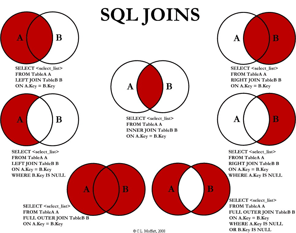
- A Visual Explanation of SQL Joins - Coding Horror
-
http://publib.boulder.ibm.com/infocenter/iseries/v5r4/index.jsp?topic=%2Fsqlp%2Frbafyjoin.htm
- Inner Join (ANSI supported)
- Records in both table A and table B where the given condition matches. e.g,
SELECT * FROM TableA INNER JOIN TableB ON TableA.name = TableB.name
- Records in both table A and table B where the given condition matches. e.g,
- Cross Join (ANSI supported)
- Every possible pair of rows from both the tables. Basically a cartesian product
- If no condition is provided in Inner join, then it becomes a cross join. e.g.,
SELECT * FROM TableA CROSS JOIN TableB
- Left Outer Join (ANSI supported)
- produces a complete set of records from Table A, with the matching records (where available) in Table B. If there is no match, the right side will contain null.
- e.g.,
SELECT * FROM TableA LEFT OUTER JOIN TableB ON TableA.name = TableB.name
- Right Outer Join (ANSI supported)
- e.g.,
SELECT * FROM TableA RIGHT OUTER JOIN TableB ON TableA.name = TableB.name
- e.g.,
- Full Outer Join (ANSI supported)
- Full Outer Join = Left Outer + Right Outer. e.g.,
SELECT * FROM TableA FULL OUTER JOIN TableB ON TableA.name = TableB.name
- Full Outer Join = Left Outer + Right Outer. e.g.,
- Outer Join
- Records NOT in table A and table B where the given condition matches. e.g,
SELECT * FROM TableA FULL OUTER JOIN TableB ON TableA.name = TableB.name WHERE TableA.id IS null OR TableB.id IS null
- Records NOT in table A and table B where the given condition matches. e.g,
- Exception join - A left exception join returns only the rows from the first table that do not have a match in the second table.
- Equijoin -
- Natural Join- is an equijoin with redundant columns removed.
- Self Join -
- Projection - The project operator retrieves a subset of columns from a table, removing duplicate rows from the result.
Join Algorithms
Nested Loop Join
- when one table is small, and other table is large
- What is? The nested loops join, also called nested iteration, uses one join input as the outer input table and one as the inner input table. The outer loop consumes the outer input table row by row. For every outer row, the inner loop searches for matching rows in the inner input table.
- In the simplest case, the search scans an entire table or index; this is called a naive nested loops join.
- If the search exploits an index, it is called an index nested loops join.
- If the index is built as part of the query plan (and destroyed upon completion of the query), it is called a temporary index nested loops join. (All these variants are considered by the query optimizer.)
- When is it effective? A nested loops join is particularly effective if the outer input is small and the inner input is preindexed and large. In many small transactions, such as those affecting only a small set of rows, index nested loops joins are superior to both merge joins and hash joins. In large queries, however, nested loops joins are often not the optimal choice.
- Block nested loop join…
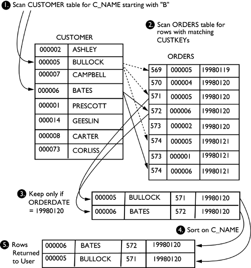
Merge Join / Sort-Merge Join
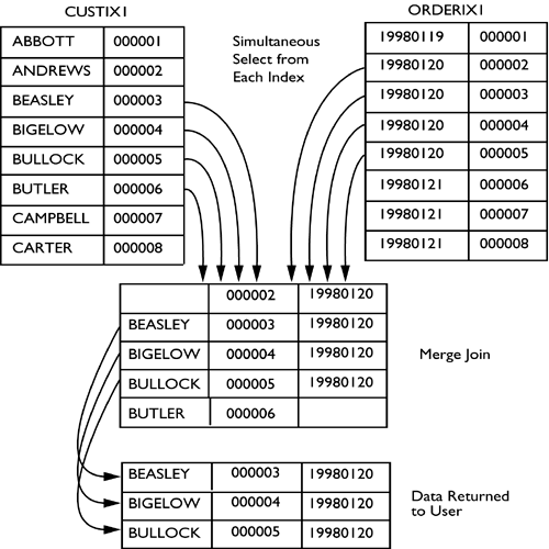
- when both the tables involved in the join are large
- The merge join requires both inputs to be sorted on the merge columns, which are defined by the equality
ONclauses of the join predicate. The query optimizer typically scans an index, if one exists on the proper set of columns, or it places a sort operator below the merge join. In rare cases, there may be multiple equality clauses, but the merge columns are taken from only some of the available equality clauses. - Because each input is sorted, the Merge Join operator gets a row from each input and compares them. For example, for inner join operations, the rows are returned if they are equal. If they are not equal, the lower-value row is discarded and another row is obtained from that input. This process repeats until all rows have been processed.
- The merge join operation may be either a regular or a many-to-many operation. A many-to-many merge join uses a temporary table to store rows. If there are duplicate values from each input, one of the inputs will have to rewind to the start of the duplicates as each duplicate from the other input is processed.
- If a residual predicate is present, all rows that satisfy the merge predicate evaluate the residual predicate, and only those rows that satisfy it are returned.
- Merge join itself is very fast, but it can be an expensive choice if sort operations are required. However, if the data volume is large and the desired data can be obtained presorted from existing B-tree indexes, merge join is often the fastest available join algorithm.
Hash Join
- when the data set is large but the result set expected is small
- This algorithm also has a startup penalty by forcing you to build a hash table of one of the input sets before the actual join can start.
- Performance
- Compared to the sort merge join this is easier as it involves only one sweep through the data and therefore the computational complexity is
O(n)while sorting won’t be better thanO(n log n). So in general you can build the hash faster than you would be able to do the sorting. - The hash also needs to be computed for only one input set and this could be the smaller one.
- This makes the hash join often the preferred choice over the sort merge join.
- Compared to the sort merge join this is easier as it involves only one sweep through the data and therefore the computational complexity is
- Generally speaking the hash join wins when you expect a large result set and the nested loop join wins when you expect a small result set. One of the most dominant problems in this area is the planner getting the estimates wrong and taking the other path.
- The hash join can only be used if you use equality as join relation.
- Building the hash needs temporary space and increasing work_mem sometimes helps.
-
The hash join is also a good candidate for parallel processing.
- Joining in DB2
- Join Methods and Strategies
- Getting the Most from Hash Joins
Administration Concepts
Tablespaces
Table spaces are logical objects used as a layer between logical tables and physical containers. Containers are where the data is physically stored in files, directories, or raw devices. When you create a table space, you can associate it to a specific buffer pool (database cache) and to specific containers.
Default Tablespaces
There are 3 table spaces created automatically when a database is created:
- Catalog (SYSCATSPACE): The catalog and the system temporary space can be considered system structures, as they are needed for the normal operation of your database. The catalog contains metadata (data about your database objects) and must exist at all times. * System temporary space (TEMPSPACE1): is the work area for the database manager to perform operations, like joins and overflowed sorts. There must be at least one system temporary table space in each database. * Default user table space (USERSPACE1): This is created by default, but you can delete it. To create a table in a given table space, use the CREATE TABLE statement with the IN table_space_name clause. If a table space is not specified in this statement, the table will be created in the first user created table space. If you have not yet created a table space, the table will be created in the USERSPACE1 table space.
Types
- System-managed space (SMS): This type of table space is managed by the operating system and requires minimal administration. This is the default table space type.
- Database-managed space (DMS): This type of table space is managed by the DB2 database manager, and it requires some administration
Buffer Pools
A buffer pool is an area in physical memory that caches the database information most recently used. Without buffer pools, every single piece of data has to be retrieved from disk, which is very slow. Buffer pools are associated to tables and indexes through a table space. A buffer pool is an area in memory where all index and data pages other than LOBs are processed.DB2 retrieves LOBs directly from disk. Buffer pools are one of the most important objects to tune for database performance.
Operational Commands
DB2
- Enter command prompt by typing ‘db2’
- To take input from a file and output to a file:
db2 -tvf db2input.txt > db2output.txt & - To connect to database:
CONNECT to NYCMRDI4 USER cmdrinfr USING s0mepassw0rd - Command to list the databases:
list db directory - Command to list the tables:
list db tables - Read input from file:
db2 -tvf filename Db2advis- command to advice indexes on sql-
Reorg
- Check transaction log usage :
call sp.xlogfull() - Row count on table without full table scan
1
| |
- Truncate a table without transaction logging
1
| |
This operation is fully recoverable. Note that on Windows systems, you have to replace /dev/null by NUL.
OR
1
| |
Causes all data currently in table to be removed. Once the data has been removed, it cannot be recovered except through use of the RESTORE facility. If the unit of work in which this alter statement was issued is rolled back, the table data will not be returned to its original state. When this action is requested, no DELETE triggers defined on the affected table are fired. Any indexes that exist on the table are also deleted.
- Dummy select
1
| |
Bibliography
- Physical Database Design - The Database Professional’s Guide to Exploiting Indexes, Views, Storage, and More
- Refactoring Databases
- SQL Anti-patterns
- http://www.geekinterview.com/articles/sql-interview-questions-with-answers.html